In data analytics we come across the term “Regression” very frequently. Before we continue to focus topic i.e. “Linear Regression” lets first know what we mean by Regression. Regression is a statistical way to establish a relationship between a dependent variable and a set of independent variable(s). e.g., if we say that

Age = 5 + Height * 10 + Weight * 13

Here we are establishing a relationship between Height & Weight of a person with his/ Her Age. This is a very basic example of Regression.

Introduction

Least Square “Linear Regression” is a statistical method to regress the data with dependent variable having continuous values whereas independent variables can have either continuous or categorical values. In other words “Linear Regression” is a method to predict dependent variable (Y) based on values of independent variables (X).  It can be used for the cases where we want to predict some continuous quantity. E.g., Predicting traffic in a retail store, predicting a user’s dwell time or number of pages visited on Dezyre.com etc.

Prerequisites

To start with Linear Regression, you must be aware of a few basic concepts of statistics. i.e.,

Assumptions of Linear Regression

Not a single size fits or all, the same is true for Linear Regression as well. In order to fit a linear regression line data should satisfy few basic but important assumptions. If your data doesn’t follow the assumptions, your results may be wrong as well as misleading.

Get Closer To Your Dream of Becoming a Data Scientist with 70+ Solved End-to-End ML Projects

Linear Regression Line

While doing linear regression our objective is to fit a line through the distribution which is nearest to most of the points. Hence reducing the distance (error term) of data points from the fitted line.

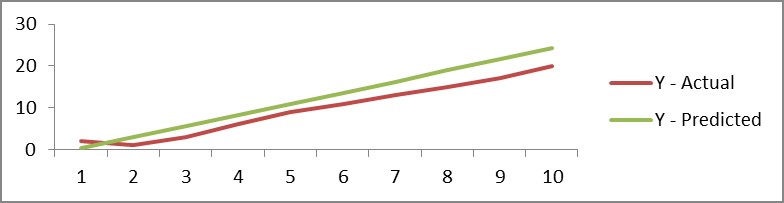
For example, in above figure (left) dots represent various data points and line (right) represents an approximate line which can explain the relationship between ‘x’ & ‘y’ axes. Through, linear regression we try to find out such a line. For example, if we have one dependent variable ‘Y’ and one independent variable ‘X’ – relationship between ‘X’ & ‘Y’ can be represented in a form of following equation:

Y = Β0 + Β1X

Where,

Food for thought: Why to reduce “Square of errors” and not just the errors?

Food for thought: Will correlation coefficient between ‘X’ and ‘Y’ be same as Β1?

Get FREE Access to Machine Learning Example Codes for Data Cleaning, Data Munging, and Data Visualization

Using a statistical tool e.g., Excel, R, SAS etc. you will directly find constants (B0 and B1) as a result of linear regression function. But conceptually as discussed it works on OLS concept and tries to reduce the square of errors, using the very concept software packages calculate these constants.

For example, let say we want to predict ‘y’ from ‘x’ given in following table and let’s assume that our regression equation will look like “y=B0+B1*x”

x

y

Predicted 'y'

1

2

Β0+B1*1

2

1

Β0+B1*2

3

3

Β0+B1*3

4

6

Β0+B1*4

5

9

Β0+B1*5

6

11

Β0+B1*6

7

13

Β0+B1*7

8

15

Β0+B1*8

9

17

Β0+B1*9

10

20

Β0+B1*10

Table 1:

Std. Dev. of x

3.02765

Std. Dev. of y

6.617317

Mean of x

5.5

Mean of y

9.7

Correlation between x & y

.989938

If we differentiate the Residual Sum of Square (RSS) wrt. B0 & B1  and equate the results to zero, we get the following equations as a result:        

B1 = Correlation * (Std. Dev. of y/ Std. Dev. of x)

B0 = Mean(Y) – B1 * Mean(X)

Putting values from table 1 into the above equations,

B1 = 2.64

B0 = -2.2

Hence, the least regression equation will become –

Y = -2.2 + 2.64*x

Let see, how our predictions are looking like using this equation

x

Y - Actual

Y - Predicted

1

2

0.44

2

1

3.08

3

3

5.72

4

6

8.36

5

9

11

6

11

13.64

7

13

16.28

8

15

18.92

9

17

21.56

10

20

24.2

Once you build the model, the next logical question comes in mind is to know whether your model is good enough to predict in future or the relationship which you built between dependent and independent variables is good enough or not.

For this purpose there are various metrics which we look into-

R – Square (R2)

Formula for calculating R2 is given by:

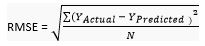
Where N is the number of observations used to fit the model, σx is the standard deviation of x, and σy is the standard deviation of y.

Recommended Tutorials:

RMSE tells the measure of dispersion of predicted values from actual values. The formula for calculating RMSE is

N : Total number of observations

Though RMSE is a good measure for errors but the issue with it is that it is susceptible to the range of your dependent variable. If your dependent variable has thin range, your RMSE will be low and if dependent variable has wide range RMSE will be high. Hence, RMSE is a good metric to compare between different iterations of a model.

To overcome the limitations of RMSE, analyst prefer MAPE over RMSE which gives error in terms of percentages and hence comparable across models. Formula for calculating MAPE can be written as:

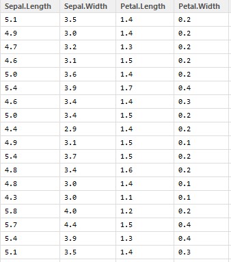
N : Total number of observations

Learn Data Science by working on interesting Data Science Projects 

Till now we were discussing about the scenario where we have only one independent variable. If we have more than one independent variable the procedure for fitting a best fit line is known as “Multiple Linear Regression”

Fundamentally there is no difference between ‘Simple’ & ‘Multiple’ linear regression. Both works on OLS principle and procedure to get the best line is also similar. In the case of later, regression equation will take a shape like:

 Y=B0+B1X1+B2X2+B3X3.....

Where,

Let’s take a case where we have to predict ‘Petal.Width’ from the given data set ( We are using ‘iris’ dataset which comes along with R). We will be using R as a platform to run the regression on our dataset (If you are not familiar with R, you can use Microsoft Excel as well for your learning purpose). Firstly, let see how data looks like-

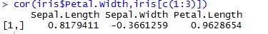
We can see that there are 4 variables in our data out of which Petal.Width is a dependent variable while rests of them are predictors or independent variables. Now, let’s calculate correlation between our dependent & independent variables:

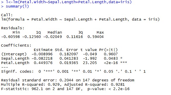
Explore More Data Science and Machine Learning Projects for Practice. Fast-Track Your Career Transition with ProjectPro

From the correlation matrix we can see that not all the variables are strongly correlated to Petal.Width, hence we will only include significant variables to build our model i.e. ‘Sepal.Length’ & ‘Petal.Length’. Let’s run our first model:

Here, Intercept estimate is same as B0 in previous examples, while coefficient values written next to the variable names are nothing but our beta coefficients (B1, B2, B3 …. Etc.). Hence we can write our linear regression equation as:

Petal.Width = -0.008996 – 0.082218*Sepal.Length + 0.449376*Petal.Length

When we run a linear regression, there is an underlying assumption that there is some relationship between dependent and independent variable. To validate this assumption, linear regression module validates the hypothesis that “Beta coefficient Bi for an independent variable Xi is 0”. The P-Value which we are seeing in the last column is nothing but the probability of this hypothesis being true. Generally if P-Value is less than or equal to 0.05 we consider this hypothesis to be false and establish a relationship between dependent and independent variable

Multi-collinearity tells us the strength of relationship between independent variables. If there is Multi-Collinearity in our data, our beta coefficients may be misleading. VIF (Variance Inflation Factor) is used to identify the Multi-collinearity. If VIF value is greater than 4 we exclude that variable from our model building exercise

Access Data Science and Machine Learning Project Code Examples

Model building is not one step process, one need to run multiple iterations in order to reach a final model. Take care of P-Value and VIF for variable selection and R-Square & MAPE for model selection.

PREVIOUS

NEXT